Color Palettes in HCL Space
This is a quick follow-up to my previous post about Color Palettes in RGB Space. Achim Zeileis had commented that, perhaps, it would be more informative to evaluate the color palettes in HCL (polar LUV) space, as that spectrum more accurately describes how humans perceive color. Perhaps more clear trends would emerge in HCL space, or color palettes would more closely hug their principal component. For the uninitiated, a good introduction to HCL color spaces is available at this site, or from Mr. Zeileis' own paper here. We'll start by loading in some code written previously (or slightly modified to support HCL). We can plot out an image of the different color palettes we're evaluating once again.
source("../Correlation.R")
source("loadPalettes.R")
par(mfrow = c(6, 3), mar = c(2, 1, 1, 1))
for (i in 1:18) {
    palette <- getSequentialLuv(i, allSequential)
    image(mat, col = hex(palette), axes = FALSE, main = i)
}
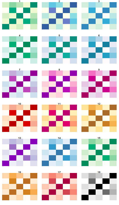
HCL-Space The fundamental question for this analysis was how these color palettes move through HCL space, as opposed to RGB space, which was considered last time.

You must enable Javascript to view this page properly.
R2 Values As we did in the previous analysis, we can use the principal component of each palette, to compute the R
2 value to quantify how well the data aligns to this component.

You must enable Javascript to view this page properly.
We'll recycle some of the old functions, and create a new one that calculates the R
2 values in HCL space.
#' Compute the proportion of variance accounted for by the given number of components
#'
#' @author Jeffrey D. Allen email{Jeffrey.Allen@@UTSouthwestern.edu}
propVar <- function(pca, components=1){
  #proportion of variance explained by the first component
  pv <- pca$sdev^2/sum(pca$sdev^2)[1]
  return(sum(pv[1:components]))
}

#' Calculate the R-squared values of all 18 color palettes
#'
#' @author Jeffrey D. Allen email{Jeffrey.Allen@@UTSouthwestern.edu}
calcR2Sequential <- function(){
  library(rgl)
  R2 <- list()
  for (i in which(sequential[,2] == 9)){
    palette <- RGBToLuv(sequential[i:(i+8), 7:9])
    pca <-plotLuvCols(palette[,"L"],palette[,"C"], palette[,"H"], pca=1)
    R2[[length(R2)+1]] <- propVar(pca,1)
  }
  return(R2)
}

calcR2RGBSequential <- function() {
    library(rgl)
    R2 <- list()
    for (i in which(sequential[, 2] == 9)) {
        palette <- sequential[i:(i + 8), 7:9]
        pca <- plotCols(palette$R, palette$G, palette$B, pca = 1)
        cat(i, ": ", propVar(pca, 1), "n")
        R2[[length(R2) + 1]] <- propVar(pca, 1)
    }
    return(R2)
}
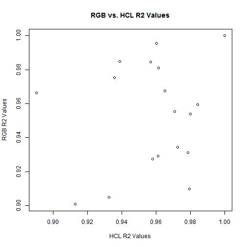
Comparison of R2 Values Let's compare the R
2 values computed from RGB space to those computed in HCL space
# R2 Values in HCL Space
r2 <- calcR2Sequential()
r2 <- unlist(r2)
names(r2) <- 1:18

# R2 Values in RGB Space
rgbr2 <- calcR2RGBSequential()
## 34 :  0.981
## 76 :  0.9097
## 118 :  0.9541
## 160 :  0.9847
## 202 :  0.9552
## 244 :  0.9663
## 286 :  0.9674
## 328 :  0.9273
## 370 :  0.9344
## 412 :  0.9593
## 454 :  0.9049
## 496 :  0.9007
## 538 :  0.9954
## 580 :  0.9752
## 622 :  0.9846
## 664 :  0.9292
## 706 :  0.9311
## 748 :  1
rgbr2 <- unlist(rgbr2)
names(rgbr2) <- 1:18

# plot the comparison
plot(rgbr2 ~ r2, ylab = "RGB R2 Values", xlab = "HCL R2 Values", main = "RGB vs. HCL R2 Values")
pv <- anova(lm(rgbr2 ~ r2))$"Pr(>F)"[1]
As seen clearly in the plot, these two variables are not correlated (p-value of
0.5232), so there's definitely a difference in how these palettes move through HCL vs. RGB space.
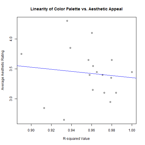
Color Ratings One hypothesis of this analysis was that because HCL space corresponds more directly to our perception of color, perhaps a smoother or more linear path through HCL space would have greater consequence on the visual appeal of the color palette than it would in RGB space. To test this, we can repeat the same analysis as we had before to see if a small R
2 value is significantly correlated with the visual appeal of a color palette.
colorPreference <- read.csv("../turk/output/Batch_790445_batch_results.csv",
    header = TRUE, stringsAsFactors = FALSE)
colorPreference <- colorPreference[, 28:29]
colorPreference[, 1] <- substr(colorPreference[, 1], 44, 100)
colorPreference[, 1] <- substr(colorPreference[, 1], 0, nchar(colorPreference[,
    1]) - 4)
colnames(colorPreference) <- c("palette", "rating")

prefList <- split(colorPreference[, 2], colorPreference[, 1])
prefList <- prefList[order(as.integer(names(prefList)))]
R2 Values We can calculate the R
2 values for each palette as previously discussed and compare to see if it's associated with the aesthetic appeal of a palette.
r2
##      1      2      3      4      5      6      7      8      9     10
## 0.9614 0.9794 0.9799 0.9388 0.9708 0.8902 0.9651 0.9579 0.9725 0.9842
##     11     12     13     14     15     16     17     18
## 0.9325 0.9129 0.9603 0.9358 0.9568 0.9611 0.9785 1.0000
plot(avgs ~ r2, main = "Linearity of Color Palette vs. Aesthetic Appeal", xlab = "R-squared Value",
    ylab = "Average Aesthetic Rating")
abline(lm(avgs ~ r2), col = 4)
pv <- anova(lm(avgs ~ r2))$"Pr(>F)"[1]
Oddly, this result contradicts the previous result; it seems that adhering to a linear path through HCL space is actually
inversely related with the aesthetic appeal on these palettes. We should note, of course, that the p-value for this correlation is not significant, as it stands (p-value = 0.6598). Regardless, the negative trend seems fairly obvious on inspection and, if you were to exclude the two "outlier" palettes on the left side which have stark breaks in HCL space on either end of the spectrum, you get a significant (0.01) negative correlation. Indeed, these same two palettes were the same outliers in the previous plot comparing RGB to HCL R2 values. Obviously, as it stands, the conclusion of the analysis is that there is no correlation in these palettes between linearity in HCL space and aesthetic appeal, but it is curious that the hinted correlation is actually negative.
Dimensional Spread Another point of interest is the "spread" or coverage of a palette across one particular axis. For instance, it may be interesting to compare a color palette which varies only in luminance to one which varies only in chroma to see if one type of progression is more aesthetically appealing. We can summarize such a phenomenon by calculating the distance between each color in a palette along a given axis (luminosity, for instance), which we'll label "ΔLuminosity" the . Extracting the median of these points may provide some insight into the movement of a particular palette along an axis.
plotDimensionalScoring <- function(palettes, scoring, ...) {

    ranges <- data.frame(L = numeric(0), C = numeric(0), H = numeric(0))

    for (i in 1:length(palettes)) {
        colPal <- RGBToLuv(palettes[[i]])

        # get the differences between each color on each axis
        colPal <- diff(colPal)
        colPal <- abs(apply(colPal, 2, median))

        ranges[i, ] <- colPal

    }

    plot3d(0, 0, 0, xlab = "L", ylab = "C", zlab = "H", type = "n", xlim = c(-0.5,
        max(ranges[, 1] + 1)), ylim = c(-0.5, max(ranges[, 2] + 1)), zlim = c(-0.5,
        max(ranges[, 3] + 1)), ...)

    cols <- heat_hcl(n = 101)

    for (i in 1:nrow(ranges)) {
        plot3d(ranges[i, 1], ranges[i, 2], ranges[i, 3], type = "p", add = TRUE,
            pch = 19, size = 10, col = cols[101 - (round(scoring[i], 2) * 100)],
            ...)
    }
    ranges
}

normAvgs <- avgs - min(avgs)
normAvgs <- normAvgs/max(normAvgs)
ranges <- plotDimensionalScoring(allSequential, normAvgs)
Each palette now has one median Δ value for each axis. We can plot these in 3D space to see where the palettes fall. We'll go ahead and color-code these based on their average visual appeal to see if we can observe any trends or "hotspots" in which palettes are consistently rated as visually appealing based only on their median movement along an axis.

You must enable Javascript to view this page properly.
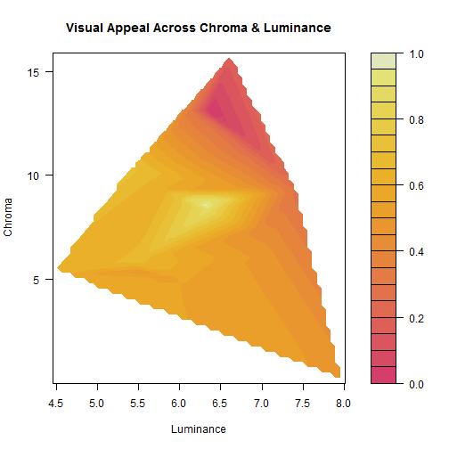
We're descending into fairly non-scientific analysis here, but I noticed a pattern when viewing these points along the chroma and luminosity axes. It seems like there's something of a pattern resulting in consistently positioned high-ranked palettes. I interpolated a heatmap based on these ratings on the C and L axes.
library(akima)

resolution = 64
cSeq <- seq(min(ranges[, 2]), max(ranges[, 2]), length.out = resolution)
lSeq <- seq(min(ranges[, 1]), max(ranges[, 1]), length.out = resolution)

a <- interp(x = ranges[, 1], y = ranges[, 2], z = normAvgs, xo = lSeq, yo = cSeq,
    duplicate = "mean")

filled.contour(a, color.palette = heat_hcl, xlab = "Luminance", ylab = "Chroma",
    main = "Visual Appeal Across Chroma & Luminance")
maxL <- lSeq[which.max(apply(a$z, 2, max, na.rm = TRUE))]
## Warning: no non-missing arguments to max; returning -Inf
maxC <- cSeq[which.max(apply(a$z, 1, max, na.rm = TRUE))]
## Warning: no non-missing arguments to max; returning -Inf
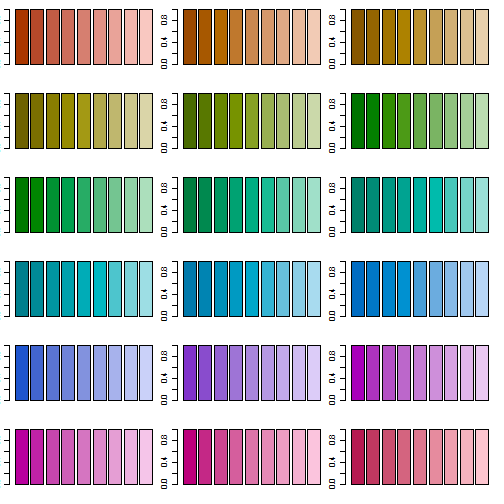
You can see the peak of visual appeal at luminance =
6.374 and chroma = 8.332. A few examples of palettes using this "optimized" chroma and luminance spacing...
par(mfrow = c(6, 3), mar = c(2, 1, 1, 1))
for (i in 1:18) {
    barplot(rep(1, 9), col = sequential_hcl(9, h = (20 * i), c. = c(100, 33.6),
        l = c(40, 84.59), power = 1))
}
Individual Axis Analysis There is one palette that seems to be a bit of an outlier in most regards. Of all the palettes, the greyscale palette has the lightest L value, and the lowest C and H values. If you calculate the Z-scores on each color axis, this palette has consistently higher scores; below is a plot of the average Z-score across the 3 axes.
barplot(apply(abs(scale(ranges)), 1, mean), col = c(rep("#BBBBBB", 17), "#CC7777"),
    xlab = "Palette #", ylab = "Average Z-score Across {H, C, L} Axes")
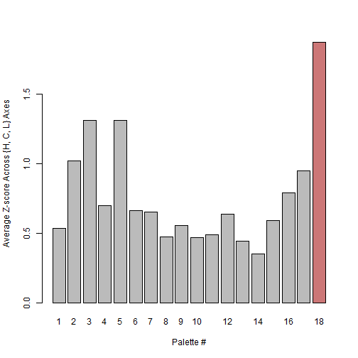
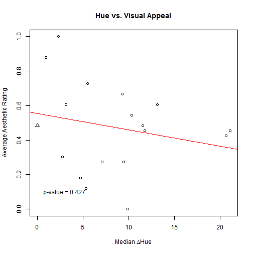
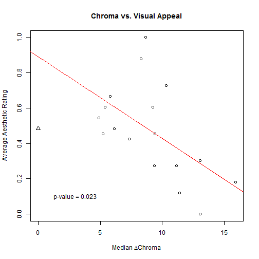
Because of this, I decided to exclude it from all further calculations of significance. Where appropriate, I'll still plot it graphically but distinguish it from the other palettes. Rather than relying on a 3D plot, we can examine each axis individually to see if there's a significant association between a palette's median variation on that access and its visual appeal. (The greyscale plot will be plotted with a triangle symbol in these plots, and was excluded to p-value and regression calculations).
filRanges <- ranges[1:17, ]
filNormAvgs <- normAvgs[1:17]

plot(normAvgs ~ ranges[, "H"], pch = c(rep(1, 17), 2), main = "Hue vs. Visual Appeal",
    xlab = expression("Median " * Delta * Hue), ylab = "Average Aesthetic Rating")
abline(lm(filNormAvgs ~ filRanges[, "H"]), col = 2)
pvH <- anova(lm(filNormAvgs ~ filRanges[, "H"]))$"Pr(>F)"[1]
text(3, 0.1, paste("p-value =", round(pvH, 3)))
plot(normAvgs ~ ranges[, "C"], pch = c(rep(1, 17), 2), main = "Chroma vs. Visual Appeal",
    xlab = expression("Median " * Delta * Chroma), ylab = "Average Aesthetic Rating")
abline(lm(filNormAvgs ~ filRanges[, "C"]), col = 2)
pvC <- anova(lm(filNormAvgs ~ filRanges[, "C"]))$"Pr(>F)"[1]
text(3, 0.1, paste("p-value =", round(pvC, 3)))
plot(normAvgs ~ ranges[, "L"], pch = c(rep(1, 17), 2), main = "Luminance vs. Visual Appeal",
    xlab = expression("Median " * Delta * Luminance), ylab = "Average Aesthetic Rating")
abline(lm(filNormAvgs ~ filRanges[, "L"]), col = 2)
pvL <- anova(lm(filNormAvgs ~ filRanges[, "L"]))$"Pr(>F)"[1]
text(5, 0.1, paste("p-value =", round(pvL, 3)))
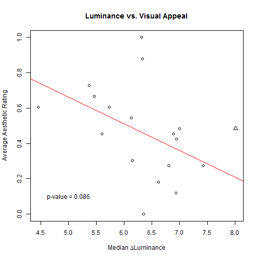
As shown on the plots, there is no observable correlation with regards to movement through hue with visual appeal; there is a significant negative correlation between median variation in chroma and the visual appeal; and there seems to be a negative (though non-significant) correlation between median variation in luminance and visual appeal.
Conclusion
Comparison to Colorspace Palettes It was mentioned that colorspace generates their palettes in HCL space, so the trends should more obviously emerge for such palettes. As it turns out, the palettes in HCL not necessarily linear, even in HCL space. Many palettes are fairly linear on at least one axis, but often have at least one color at either end which is completely non-linear, causing the R2 values to often be lower than they were in colorbrewer palettes. For instance:
csp <- as(hex2RGB(sequential_hcl(n = 9)), "polarLUV")@coords
pca <- plotLuvCols(csp[, "L"], csp[, "C"], csp[, "H"], 1)

You must enable Javascript to view this page properly.
After inspecting the code, the hue value in this color palette never changes. So it seems that we're encountering a substantial rounding error when you get the the dark/light edges of the color palette.
Summary I'm still a bit perplexed by the results I observer, but I suppose this analysis hints at a few things. First of all, I realized that it very much matters which color space you're working in when designing color palettes. As the lack of a correlation between the R
2 values from RGB space and HCL space show, the movement of different palettes through these spaces are drastically different and don't seem to be correlated. Second, it looks like there is some potential to optimize the spacing of colors in a given palette by finding these "hotspots" in the Luminance vs. Chroma plot. On the other hand, movement along the hue axis for a given palette doesn't seem to have much of an effect on the visual appeal. Finally, it seems that the rounding error on hex codes and 255-value RGB values becomes significant for especially dark or bright ends of a palette. This may put into question the effectiveness of such analysis in 3D space. Of course, the hue value represents a complete circle, so a hue of 359 is very close to a hue of 0, which wouldn't be captured in a naive 3D analysis. Even accounting for this problem, there are other nuances of this color space which can't be captured in 3D space, and may jeopardize the effectiveness of PCA in such a space.
Future Work As mentioned previously, it will be interesting to analyze not just the visual appeal of a color palette, but the effectiveness of a palette at communicating information. Hopefully the next post will be able to capture some of that information. As always, comments are welcome! I'm well outside the scope of my training and expertise, so I'd be happy to hear any critiques or concerns about methodology.
Acknowledgements
- All analysis done in R
- All ratings generated using Amazon Mechanical Turk
- Interactive 3D graphics generated using rgl version 0.92.879
- Report generated using knitr
- Code hosted by GitHub in trestletech/RGB-Space
- Color palettes obtained from Cynthia Brewer's ColorBrewer2.0 service
- Idea from Achim Zeileis
