Introduction I've recently been interested in how to communicate information using color. I don't know much about the field of Color Theory, but it's an interesting topic to me. The selection of color palettes, in particular, has been a topic I've been faced with lately.

I downloaded 18 different sequential color palettes from Cynthia Brewer's ColorBrewer2 website to use as suggested color palettes. I was struck by the various movements through the spectrum of some of these palettes and wanted to poke around at quantifying some of that movement. This is the result of that analysis.

Using the 18 different sequential color palettes, I generated heatmaps to try to gauge the aesthetic appeal of each palette. Using Amazon's Mechanical Turk, I was able to ask workers to rate a palette on a scale from 1 to 5. I had each palette rated 20 times to generate a sufficient amount of data to start determining statistical significance. The 360 ratings were completed by 28 workers in a couple of hours.

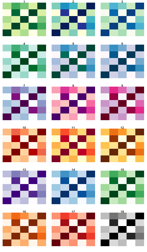
This initial study didn't consider anything about how clear the heatmaps are, only how aesthetically pleasing they are. The 18 matrices in the 18 available palettes are displayed below.

  source("../Correlation.R")
  source("loadPalettes.R")
  par(mfrow = c(6, 3), mar = c(2, 1, 1, 1))
  for (i in 1:18) {
      palette <- allSequential[[i]]
      image(mat, col = rgb(palette/255), axes = FALSE, main = i)
  }
  

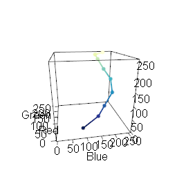
RGB-Space One question I had was about the motion of a "visually attractive" color palette through the 3-dimensional space of all RGB values. My assumption was that most palettes can be represented as a straight line through

Your browser does not support the HTML5 canvas element.

You must enable Javascript to view this page properly.

An interactive visualization of palette #2 in 3-Dimensional RGB space

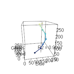
R² Values One way to quantify this is to calculate the principal component of each palette, which represents the line in RGB space which best fits the palette. The R

² value can then be used to quantify how well the data aligns to this component. An R² value of 1 indicates that the palette aligns perfectly to a straight line through RGB space.

Your browser does not support the HTML5 canvas element.

You must enable Javascript to view this page properly.

Palette #2 with the Principal Component. Note the curve of the palette around the component.

  #' Compute the proportion of variance accounted for by the given number of
  #' components
  #' 
  #' @author Jeffrey D. Allen \email{jeff.allen@@trestletech.com}
  propVar <- function(pca, components = 1) {
      # proportion of variance explained by the first component
      pv <- pca$sdev^2/sum(pca$sdev^2)[1]
      return(sum(pv[1:components]))
  }
  
  #' Calculate the R-squared values of all 18 color palettes
  #' 
  #' @author Jeffrey D. Allen \email{jeff.allen@@trestletech.com}
  calcR2Sequential <- function() {
      library(rgl)
      R2 <- list()
      for (i in which(sequential[, 2] == 9)) {
          palette <- sequential[i:(i + 8), 7:9]
          pca <- plotCols(palette$R, palette$G, palette$B, pca = 1)
          cat(i, ": ", propVar(pca, 1), "\n")
          R2[[length(R2) + 1]] <- propVar(pca, 1)
      }
      return(R2)
  }
  

Path Length An alternative way to consider the palette in RGB space is to consider the "length" of the palette through RGB space by simply calculating the distance between each color represented as a point in RGB space. My thought is that this may better capture the "movement" of a palette around this space. The R

² value doesn't encompass any notion of how much space is covered by a palette, but only the arrangement of the colors relative to their principal component.

  #' Calculate the path length for all sequential palettes.
  #' 
  #' @author Jeffrey D. Allen \email{jeff.allen@@trestletech.com}
  calcPathLength <- function() {
      plen <- array(dim = sum(sequential[, 2] == 9, na.rm = TRUE))
      p <- 1
      for (i in which(sequential[, 2] == 9)) {
          palette <- sequential[i:(i + 8), 7:9]
          cat(i, ": ", getPathLength(palette), "\n")
          plen[p] <- getPathLength(palette)
          p <- p + 1
      }
      return(plen)
  }
  
  #' Calculate the length of a path through RGB space of a given palette.
  #' 
  #' Sums the distance from all adjacent colors.  @author Jeffrey D. Allen
  #' \email{jeff.allen@@trestletech.com}
  getPathLength <- function(palette) {
      pd <- apply(palette, 2, diff)
      pl <- sqrt(apply(pd^2, 1, sum))
      return(sum(pl))
  }
  

Comparison Let's compare the R

² values to the path length values

  r2 <- calcR2Sequential()
  



  ## 34 :  0.981 
  ## 76 :  0.9097 
  ## 118 :  0.9541 
  ## 160 :  0.9847 
  ## 202 :  0.9552 
  ## 244 :  0.9663 
  ## 286 :  0.9674 
  ## 328 :  0.9273 
  ## 370 :  0.9344 
  ## 412 :  0.9593 
  ## 454 :  0.9049 
  ## 496 :  0.9007 
  ## 538 :  0.9954 
  ## 580 :  0.9752 
  ## 622 :  0.9846 
  ## 664 :  0.9292 
  ## 706 :  0.9311 
  ## 748 :  1 
  



  r2 <- unlist(r2)
  names(r2) <- 1:18
  
  pl <- calcPathLength()
  



  ## 34 :  404.8 
  ## 76 :  455.2 
  ## 118 :  377.5 
  ## 160 :  407.5 
  ## 202 :  418.1 
  ## 244 :  400.5 
  ## 286 :  389.5 
  ## 328 :  405.6 
  ## 370 :  430 
  ## 412 :  420.7 
  ## 454 :  424.7 
  ## 496 :  430 
  ## 538 :  342.9 
  ## 580 :  374.1 
  ## 622 :  400.2 
  ## 664 :  400.3 
  ## 706 :  430.6 
  ## 748 :  441.7 
  



  plot(r2 ~ pl, main = "Path Length vs. R-Squared Value", xlab = "Path Length",
      ylab = "R-Squared Value")
  abline(lm(r2 ~ pl), col = 2)
  






  pv <- anova(lm(r2 ~ pl))$"Pr(>F)"[1]
  

The p-value (

0.0318) is significant in the negative correlation between the two variables, meaning that, as expected, the closer the palette stays to its principal component, the shorter the path through RGB space is (on average). So either scheme could be used to quantify a palette's non-linearity.

Color Ratings The output of the Mechanical Turk trial is available in a stored file in this project. We'll read it in and filter out the peripheral information.

  colorPreference <- read.csv("../turk/output/Batch_790445_batch_results.csv",
      header = TRUE, stringsAsFactors = FALSE)
  colorPreference <- colorPreference[, 28:29]
  colorPreference[, 1] <- substr(colorPreference[, 1], 44, 100)
  colorPreference[, 1] <- substr(colorPreference[, 1], , nchar(colorPreference[,
      1]) - 4)
  colnames(colorPreference) <- c("palette", "rating")
  
  prefList <- split(colorPreference[, 2], colorPreference[, 1])
  prefList <- prefList[order(as.integer(names(prefList)))]
  

We can then visualize the results, as well.

  boxplot(prefList, main = "Ratings of Color Palettes", xlab = "Palette Number",
      ylab = "Rating")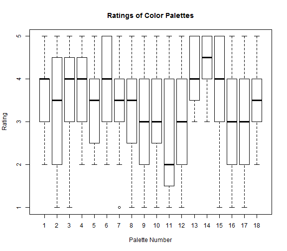
  






  avgs <- sapply(prefList, mean)
  

We can then check to see if there's a significant association between the palette and the rating of the palette, or if we've just got noise.

  fit <- anova(lm(colorPreference[, 2] ~ as.factor(colorPreference[,
      1])))
  pv <- (fit$"Pr(>F)")[1]
  

With a p-value of

1.6911 × 10<sup>-4</sup>, you can see that there is a significant difference between the different palettes.

We can list out the most attractive palettes in order, as well:

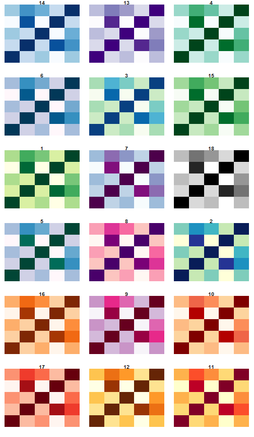
  sort(sapply(prefList, mean), decreasing = TRUE)
  



  ##   14   13    4    6    3   15    1    7   18    5    8    2   16    9   10 
  ## 4.30 4.10 3.85 3.75 3.65 3.65 3.55 3.45 3.45 3.40 3.40 3.35 3.15 3.10 3.10 
  ##   17   12   11 
  ## 2.95 2.85 2.65 
  

So the palettes, in order of visual appeal are:

  par(mfrow = c(6, 3), mar = c(2, 1, 1, 1))
  for (i in order(avgs, decreasing = TRUE)) {
      palette <- allSequential[[i]]
      image(mat, col = rgb(palette/255), axes = FALSE, main = i)
  }
  

Warm Palettes The first thing I noticed was that the cooler palettes were rated more highly than the warmer palettes. To try to quantify this, we can plot out the "redness" (the strenght of the red channel in each palette) against the average rating.

  redness <- apply(sapply(allSequential, "[[", "R"), 2, mean)
  plot(avgs ~ redness, main = "Warmth of Palette vs. Aesthetic Appeal",
      xlab = "\"Redness\"", ylab = "Average Aesthetic Rating")
  abline(lm(avgs ~ redness), col = 2)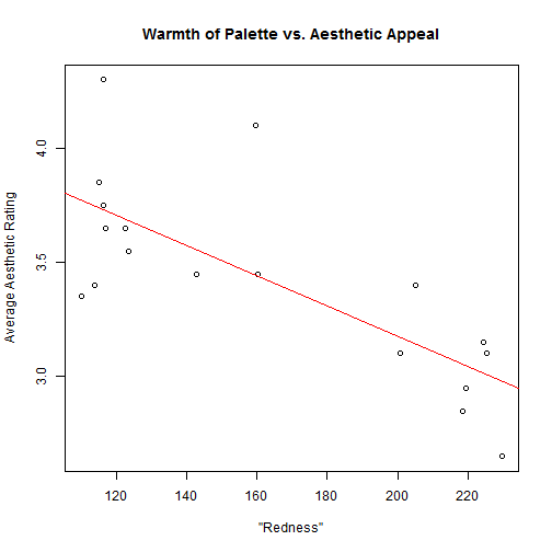
  






  pv <- anova(lm(avgs ~ redness))$"Pr(>F)"[1]
  

Indeed, the p-value of this correlation is significant for this data (

3.6602 × 10<sup>-4</sup>) indicating that -- among these palettes and in this context -- cooler palettes are more visually appealing.

R² Values We can calculate the R

² values for each palette as previously discussed and compare to see if it's associated with the aesthetic appeal of a palette.

  r2
  



  ##      1      2      3      4      5      6      7      8      9     10 
  ## 0.9810 0.9097 0.9541 0.9847 0.9552 0.9663 0.9674 0.9273 0.9344 0.9593 
  ##     11     12     13     14     15     16     17     18 
  ## 0.9049 0.9007 0.9954 0.9752 0.9846 0.9292 0.9311 1.0000 
  



  plot(avgs ~ r2, main = "Linearity of Color Palette vs. Aesthetic Appeal",
      xlab = "R-squared Value", ylab = "Average Aesthetic Rating")
  abline(lm(avgs ~ r2), col = 4)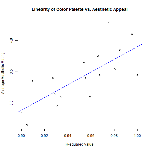
  






  pv <- anova(lm(avgs ~ r2))$"Pr(>F)"[1]
  

Again, the p-value of this association is significant (

3.2224 × 10<sup>-4</sup>). So it seems that adhering a color spectrum to a straight line through RGB-space is visually appealing.

Similarly, for the path length, the p-value is significant (though not as strongly as with the R² values).

  anova(lm(avgs ~ pl))$"Pr(>F)"[1]
  



  ## [1] 0.001476
  

Summary This analysis answered a couple of questions for me. First, it showed that, in general, linear paths through RGB space create more aesthetically pleasing color palettes. Second, it demonstrated that, in this narrow study, palettes with cooler color schemes were preferred as more "aesthetically pleasing." Finally, it gave some concrete recommendations regarding which of the available color palettes to use if the goal is purely aesthetic.

Future Work Of course, aesthetics are not to only goal behind color palette selection. Generally, the goal of heatmaps such as these is to convey information. If no legend is given, we're hoping to convey relative "strengths" of some phenomena to the viewer. If a legend is given, we're additionally hoping to support some quantification to these data, as well. So merely determining which color palettes are best to look at will likely not be the most important consideration in determining which palettes to use. We should do further analysis to determine which palettes convey such information most efficiently, and then likely make some compromise between efficient communication and aesthetics, depending on the application.

Acknowledgements

• All analysis done in R
• All ratings generated using Amazon Mechanical Turk
• Interactive 3D graphics generated using rgl version 0.92.879
• Report generated using knitr
• Code hosted by GitHub in trestletech/RGB-Space
• Color palettes obtained from Cynthia Brewer's ColorBrewer2.0 service